Example 2

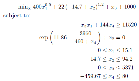
Nonlinearly constrained nonlinear program:

The above problem is a typical global optimization problem consisting of both a nonlinear objective and nonlinear constraints. As with Example 1, write anonymous functions for the objective and constraints. For multiple constraints, write the function as a column-wise vector:

% Objective Function
fun = @(x) 400*x(1)^0.9 + 22*(-14.7 + x(2))^1.2 + x(3) + 1000;

% Nonlinear Constraints
nlcon = @(x) [ x(3)*x(1) + 144*x(4);
               -exp(11.86 - 3950/(460 + x(4))) + x(2) ];
cl = [11520;0];
cu = [Inf;0];

% Bounds
lb = [0;14.7;0;-459.67];
ub = [15.1;94.2;5371;80];

% Starting Guess
x0 = [NaN;14.7;NaN;NaN];

In the above code block, we have also defined a starting guess for x2 as 14.7. For the other variables, NaN indicates to BARON to let it choose a starting point. The problem can be solved as follows:

[x,fval,exitflag,info] = baron(fun,[],[],[],lb,ub,nlcon,cl,cu,[],x0)

And the solution is:

x =

 0.0000
94.1779
 0.0001
80.0000

We can also inspect the information structure returned from BARON for more information on the solver run:

info =

   Model_Status: 'Optimal Within Tolerances'
   BARON_Status: 'Normal Completion'
     Total_Time: 0.3300
 BaR_Iterations: 13
      Best_Node: 6
Max_Nodes_InMem: 3
    Lower_Bound: 5.1949e+003
    Upper_Bound: 5.1949e+003
     Bad_Bounds: 0

This information indicates that the solver converged as expected and has bounded the objective value within the default tolerance to ensure a globally optimal solution to this model.

The MATLAB/BARON interface is provided at http://www.minlp.com. The interface is provided free of charge and with no warranties.